What is it?
Graph/network theories were first developed in physics and chemistry to quantify complex systems, such as electrical circuits and particle movements. The intuitiveness and elegance of network methodology soon captured attention from many other fields. You are likely to hear one of the following terms such as “social network,” “neural network,” “Bayesian network,” “global shipping network,” or “metabolic network.” Although the exact analytical method behind each network may vary, the foundation and mathematical theorems are largely the same.
Network analysis can be flexibly applied to any complex systems in which you have one to several types of targeted entities (e.g., individuals, behaviors, packages, symptoms, words, states, actions, neurons, atoms, you name it) that can be represented with nodes/vertices. The relationships among these nodes/vertices can be quantified and represented with edges/links. These edges/links can depict either undirected relationships, such as associations, correlations, and partial correlations, or directed relationships, such as causal inferences, predictions, causal effects, depending on the type of data you have. You can also choose to construct an unweighted (i.e., all edges have the same strength) or weighted network. These edges/links can also be dynamic and updated over time.
Why use it?
Network analysis has a lot of advantages in depicting a complex system. It can delineate various types of relationships mentioned above and accommodate multiple types of variables, such as binary, count, and continuous variables with different distribution assumptions. A network can also be updated flexibly to capture dynamic changes. It is an elegant and intuitive way to understand and represent a complex system.
When to use it?
The best timing to use network analysis is when you are interested in the patterns of relationships in a complex system or building a network that requires frequent updates of multiple edges. A single relationship in a network may not always be stable (depending on your data type). Even if it is stable, it may be hard to interpret every relationship in an extensive network. Selectively picking a few interpretable relationships for your report can easily mislead your readers (as well as yourself) and introduce enormous bias. Thus, if you are interested in a few particular relationships, you can simply apply regression analysis or other statistical tests. Also, I hope you keep in mind that the estimation of a network may be more time-consuming than you would think. You need to think through if you have incorporated all (or at least as comprehensive as possible) relevant variables into the network and check the stability of your network (which requires time-consuming resampling techniques and/or simulation tests). In sum, don’t shoot butterflies with rifles.
How to use it?
The basic: Correlation network
I will demonstrate how to build a symptom network using a subset of data from the National Epidemiologic Survey on Alcohol and Related Conditions, Second Wave (NESARC-II).
#Load data
df = read.csv('NESARC_SubstanceStress071021.csv')

#Glance the data
str(df)
## 'data.frame':    34653 obs. of  31 variables:
##  $ ID      : int  1 2 3 4 5 6 7 9 10 11 ...
##  $ Alc_A1  : int  0 0 0 0 0 0 0 0 0 0 ...
##  $ Alc_A2  : int  0 0 0 0 0 0 0 0 0 0 ...
##  $ Alc_A3  : int  0 0 0 0 0 1 0 0 0 1 ...
##  $ Alc_A4  : int  0 0 0 0 0 1 0 0 0 0 ...
##  $ Alc_A5  : int  0 0 0 0 0 0 0 0 0 0 ...
##  $ Alc_A6  : int  0 0 0 0 0 0 0 0 0 0 ...
##  $ Alc_A7  : int  0 0 0 0 0 0 0 0 0 0 ...
##  $ Alc_B1  : int  0 0 0 0 0 0 0 0 0 0 ...
##  $ Alc_B2  : int  0 0 0 0 0 0 0 0 0 0 ...
##  $ Alc_B3  : int  0 0 0 0 0 0 0 0 0 0 ...
##  $ Alc_B4  : int  0 0 0 0 0 0 0 0 0 0 ...
##  $ Tob_A1  : int  0 0 0 0 0 0 0 0 0 0 ...
##  $ Tob_A2  : int  0 0 0 0 0 0 0 0 0 1 ...
##  $ Tob_A3  : int  0 0 0 0 0 0 0 0 0 NA ...
##  $ Tob_A4  : int  0 0 0 0 0 0 0 0 0 1 ...
##  $ Tob_A5  : int  0 0 0 0 0 0 0 0 0 0 ...
##  $ Tob_A6  : int  0 0 0 0 0 0 0 0 0 0 ...
##  $ Tob_A7  : int  0 0 0 0 0 0 0 0 0 1 ...
##  $ Drug_A1 : int  0 0 0 0 0 0 0 0 0 0 ...
##  $ Drug_A2 : int  0 0 0 0 0 0 0 0 0 0 ...
##  $ Drug_A3 : int  0 0 0 0 0 0 0 0 0 0 ...
##  $ Drug_A4 : int  0 0 0 0 0 0 0 0 0 0 ...
##  $ Drug_A5 : int  0 0 0 0 0 0 0 0 0 0 ...
##  $ Drug_A6 : int  0 0 0 0 0 0 0 0 0 0 ...
##  $ Drug_A7 : int  0 0 0 0 0 0 0 0 0 0 ...
##  $ Drug_B1 : int  0 0 0 0 0 0 0 0 0 0 ...
##  $ Drug_B2 : int  0 0 0 0 0 0 0 0 1 0 ...
##  $ Drug_B3 : int  0 0 0 0 0 0 0 0 0 0 ...
##  $ Drug_B4 : int  0 0 0 0 0 0 0 0 0 0 ...
##  $ Stressor: int  2 2 0 1 3 1 2 1 7 1 ...
According to the str() function (similar to the dataframe.info()
function in Python), we know that the current data consists of 34,653
individuals with 31 variables, namely the IDs, alcohol
abuse/dependence symptoms, tobacco abuse symptoms, drug abuse/dependence
symptoms, and the number of stressors in the past year.
The symptoms are all binary variables, whereas the number of stressors is a continuous variable.
You can already see missing values in the display. Sometimes you cannot observe it directly. Always inspect missing values before you proceed to any analysis.
#Inspect missing data
require(finalfit)

df %>%
  missing_plot()
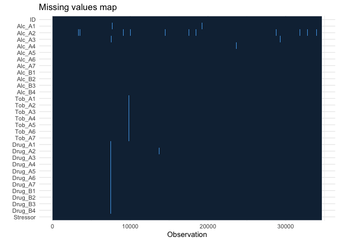 You can see that the data is not missing at random (which is often [if
not always] the case in reality). There are reasons why A2 (withdraw
symptom) had more missing values, and when one person skipped a
question, they just ignored the rest. There are many ways to deal with
missing values, but we will just use listwise deletion today.
#Listwise deletion
df_lwd = na.omit(df) #I prefer saving it as a distinct dataframe instead of rewriting the original one.
PS All blocks of code and results are horizontally scrollable.
Okay! Let’s finally do some network analysis. The most commonly used
package for network visualization in R is qgraph, which is a wrapper
of igraph. You can simply put a correlation matrix in qgraph to get
a symptom network.
require(qgraph)
qgraphSym = qgraph(cor(df_lwd[, c(2:30)]), #correlation matrix of symptoms
layout = 'spring') #Spring layout gives a force embedded layout where the distance between nodes are driven by the strength of relationships. You can use other layouts such as circle or groups.
```ss
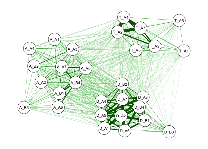
We call this a *correlation network* because the edges represent the
correlations among symptoms. Thicker edges indicate stronger
associations. You can see that, naturally, alcohol, tobacco, and drug
use symptoms become three clusters. Further, the alcohol and drug use
clusters seem to be closer to each other compared to their distance to
the tobacco cluster.
Sometimes our eyes can be deceiving, so let’s check the average distance
between symptoms of the three clusters. First, we can use the
`centrality_auto()` function to calculate different types of
[centrality](https://en.wikipedia.org/wiki/Centrality), including
betweenness, closeness, strength, expected influence, edge betweenness,
and shortest path lengths. For more discussions on centrality, see the
[article](https://arxiv.org/pdf/1209.4616.pdf) by Ghosh and Lerman
(2000).
``` r
#Calculate various types of centrailty indices
cen_qgraphSym = centrality_auto(qgraphSym)
#Save the shortest path lengths matrix
cenPath_qgraphSym = cen_qgraphSym$ShortestPathLengths
str(cenPath_qgraphSym)
##  num [1:29, 1:29] 0 3.69 2.83 2.97 2.95 ...
##  - attr(*, "dimnames")=List of 2
##   ..$ : Named chr [1:29] "A_A1" "A_A2" "A_A3" "A_A4" ...
##   .. ..- attr(*, "names")= chr [1:29] "Alc_A1" "Alc_A2" "Alc_A3" "Alc_A4" ...
##   ..$ : Named chr [1:29] "A_A1" "A_A2" "A_A3" "A_A4" ...
##   .. ..- attr(*, "names")= chr [1:29] "Alc_A1" "Alc_A2" "Alc_A3" "Alc_A4" ...
The ShortestPathLengths is a symmetric matrix of which each cell
represents the shortest path length between any two nodes. For weighted
networks, the shorted path is based on the inverse of the absolute edge
weights.
Let’s compute the average shortest length among the three clusters.
require(dplyr) #Load dplyr for dat manipulation

#Select subsets of the shortest path length matrix and compute the average shortest length between clusters
alcDrugDistance =
  mean(cenPath_qgraphSym[grep('A_', colnames(cenPath_qgraphSym)), #All rows with row names containing A_ (alcohol use symptoms)
                  grep('D_', colnames(cenPath_qgraphSym))]) #All columns with column names contains D_ (drug use symptoms)
alcTobDistance =
  mean(cenPath_qgraphSym[grep('A_', colnames(cenPath_qgraphSym)), #Alcohol use symptoms
                  grep('T_', colnames(cenPath_qgraphSym))]) #Tobacco use symptoms
drugTobDistance =
  mean(cenPath_qgraphSym[grep('D_', colnames(cenPath_qgraphSym)), #Drug use symptoms
                  grep('T_', colnames(cenPath_qgraphSym))]) #Tobacco use symptoms

cat(paste0('The average shortest length between alcohol and drug use symptoms is ', round(alcDrugDistance, 2), '\n',
      'The average shortest length between alcohol and tobacco use symptoms is ', round(alcTobDistance, 2), '\n',
      'The average shortest length between drug and tobacco use symptoms is ', round(drugTobDistance, 2), '\n'))
## The average shortest length between alcohol and drug use symptoms is 6.62
## The average shortest length between alcohol and tobacco use symptoms is 8.5
## The average shortest length between drug and tobacco use symptoms is 9.26
Our observation is thus confirmed. You can simply change the mean()
function to sd() to obtain standard deviations. With means and
standard deviations, you can easily run significant tests, such as ANOVA
or t-tests.
The advanced: EBICglasso and Ising model
Correlations are often a mess because they contain both direct and indirect relationships. For example, if you were Dagny’s friend and Dagny was John’s girlfriend, there would be an automatic correlation between you and John through Dagny without you even knowing his existence.
That is also why sometimes partial correlations can tell us a clearer story. A partial correlation, literally, is the correlation between two nodes after you partial out the correlations shared with the other nodes. The downside of using partial correlations is that we may also partial out direct shared relationships. For example, if you actually knew John and hung out with both Dagny and John a lot, only those times you hung out with John alone would count, which would lead to an underestimation of you and John’s relationship. However, one could also argue that only relationships that are above and beyond shared relationships are important. In this case, whoever goes out with John alone has a higher intimacy with him. Remember that in network analysis, we value patterns more, such that relative strength speaks more than absolute strength of relationships. Even though your relationship with John could be underestimated, we would still know that Dagny is closer to him than you do.
Alright, so let’s estimate a partial correlation network. There are a
few different ways to do so. One way is to change the graph argument
in qgraph() to graph = “pcor”. A more modern way is to use the
EBICglasso() function for parameter tuning. This function applies
l1-regularization to penalize spurious relationships and returns a more
sparse and cleaner network. It automatically checks a range of lambdas
(a regularization parameter deciding the intensity of penalties) and
selects the best model based on Extended Bayesian Information Criteria
(EBIC). You can use EBICglasso() as a separate function or specify
graph = “glasso” in the qgraph() function directly. I would suggest
taking a look at the parameters in EBICglasso() before using it.
However, the estimation of EBICglasso() is based on the assumption of
multivariate normal distributions. In other words, if the variables
are not normally distributed continuous variables, the estimation is
incorrect.
Fortunately, someone has developed another type of network estimation
for binary variables, called the Ising model. Because our symptoms
variables are binary, we will use the IsingFit package for estimation,
which, similar to EBICglasso(), can apply l1-regularization with EBIC
model selection.
#Estimate a partial correlation network using the Ising model with l1-regularization and EBIC model selection
require(IsingFit)

isingSym =
  IsingFit(df_lwd[c(1:5000), #Use the first 5000 individuals for demonstration purpose
                  c(2:30)], #Select only symptom variables,
         AND = T, #AND-rule or the OR-rule should be used to define the edges in the network
         gamma = 0.25, #A value of hyper-parameter gamma in the extended BIC,
         progressbar = F,
         plot = F
         )
## Warning: from glmnet Fortran code (error code -2); Convergence for 2th lambda
## value not reached after maxit=100000 iterations; solutions for larger lambdas
## returned

## Warning: from glmnet Fortran code (error code -2); Convergence for 2th lambda
## value not reached after maxit=100000 iterations; solutions for larger lambdas
## returned

## Warning: from glmnet Fortran code (error code -2); Convergence for 2th lambda
## value not reached after maxit=100000 iterations; solutions for larger lambdas
## returned

## Warning: from glmnet Fortran code (error code -2); Convergence for 2th lambda
## value not reached after maxit=100000 iterations; solutions for larger lambdas
## returned

## Warning: from glmnet Fortran code (error code -2); Convergence for 2th lambda
## value not reached after maxit=100000 iterations; solutions for larger lambdas
## returned

## Warning: from glmnet Fortran code (error code -2); Convergence for 2th lambda
## value not reached after maxit=100000 iterations; solutions for larger lambdas
## returned

## Warning: from glmnet Fortran code (error code -2); Convergence for 2th lambda
## value not reached after maxit=100000 iterations; solutions for larger lambdas
## returned

## Warning: from glmnet Fortran code (error code -2); Convergence for 2th lambda
## value not reached after maxit=100000 iterations; solutions for larger lambdas
## returned

## Warning: from glmnet Fortran code (error code -2); Convergence for 2th lambda
## value not reached after maxit=100000 iterations; solutions for larger lambdas
## returned
Wait! What? Warnings!? How’s that possible? I have never seen any warnings in a tutorial but my own project. Yes, I am one of you poor folks who deal with real life data. You are likely to come across warnings in real life, especially when handling clinical data. Sit tight. Don’t panic. Let’s see what these warnings mean.
First, we need to know where the warnings came from. You can remove the
pound sign in the following code to see the source code of IsingFit
and play around with the code.
#IsingFit
After doing so, you will likely find that the warnings were from the
glmnet() function, which is a function to fit GLM with
l1-regularization and can accommodate binary variables with logistic
regression.
It tests a set of lambda values starting from the maximum lambda (i.e., the smallest value for which all coefficients are zero) to the minimum one (i.e., default value 0.001 times of the maximum lambda). You can also specify how many intermediate lambdas you want to test or a customized lambda sequence for testing.
In glmnet(), if the model does not converge at a given lambda value,
it picks the best model from previously tested lambdas and return a
warning. In the current case, the model was not able to converge at the
second lambda value. Therefore, it directly returned the model with the
first lambda as no other lambda values have been tested.
This convergence problem often happens when one variable has extremely imbalanced classes, such as a lot of 0s and a few 1s. Let’s see if this is true in our case.
isingSym$lambda.values #1st lambda value = 9.900000e+35 -> models that did not converge
##  [1] 1.026446e-02 8.422784e-03 1.171962e-02 6.509399e-03 4.031019e-03
##  [6] 1.595203e-02 5.671402e-03 1.174990e-02 1.328416e-02 4.662812e-03
## [11] 1.066261e-02 1.034854e-02 9.821395e-03 7.557797e-03 7.245646e-03
## [16] 6.026736e-03 7.306218e-03 6.304695e-03 9.900000e+35 9.900000e+35
## [21] 9.900000e+35 6.815758e-03 9.900000e+35 9.900000e+35 9.900000e+35
## [26] 9.900000e+35 5.513295e-03 9.900000e+35 9.900000e+35
colMeans(df_lwd[c(1:5000), c(2:30)])
##  Alc_A1  Alc_A2  Alc_A3  Alc_A4  Alc_A5  Alc_A6  Alc_A7  Alc_B1  Alc_B2  Alc_B3
##  0.0596  0.0260  0.0728  0.0692  0.0198  0.0084  0.0310  0.0066  0.0670  0.0088
##  Alc_B4  Tob_A1  Tob_A2  Tob_A3  Tob_A4  Tob_A5  Tob_A6  Tob_A7 Drug_A1 Drug_A2
##  0.0168  0.0248  0.1714  0.0594  0.1610  0.0436  0.0234  0.1460  0.0058  0.0056
## Drug_A3 Drug_A4 Drug_A5 Drug_A6 Drug_A7 Drug_B1 Drug_B2 Drug_B3 Drug_B4
##  0.0054  0.0152  0.0094  0.0044  0.0078  0.0044  0.0144  0.0020  0.0086
We can see that the occurrence of problematic lambda values matches symptoms with low prevalence rates. This indicates that given the low prevalence rates of these symptoms, no stable relationship can be established. Thus, you will see that these drug use symptoms are not connected with other symptoms in the network shown below.
qgraph(isingSym$weiadj, layout = 'spring')
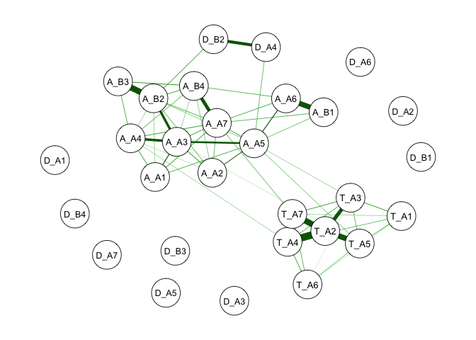
Although we need to be cautious interpreting results with warnings,
warnings do not directly sentence your model to death. There are a few
further directions you can take after a thorough inspection of the
warnings and your data. First, you can remove problematic variables.
This can also improve your estimation speed. Second, you can focus on a
subgroup of people whose variables are less imbalanced. For example, we
can directly examine a high-risk or clinical population.
Below is an example excluding drug use symptoms. You can also observe that the estimation speed improves drastically because nonconverging models require maximum times of iterations. You can compare this partial correlation network to the previous correlation network. You will find that this one is sparser and provide a clearer picture of important connections among symptoms.
singSym_AlcTob =
  IsingFit(df_lwd[c(1:5000), #Use the first 5000 individuals for example
                  c(2:18)], #Select only symptom variables ],
         AND = T, #AND-rule or the OR-rule should be used to define the edges in the network
         gamma = 0.25, #A value of hyper-parameter gamma in the extended BIC
         progressbar = F
         )
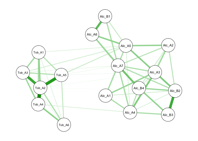
The last example is focused on a high-risk population who reported more
than seven stressors in the past year. You can see that the prevalence
rates of drug use symptoms are higher in this subgroup. As a result, we
can easily estimate partial correlations among all symptoms without
convergence issues.
#Inspect prevalence rates of symptoms in people with more than 7 stressors in the past year
colMeans(df_lwd[df_lwd$Stressor == 7, c(2:30)]) #Select people who have more than 7 stressors in the past
##     Alc_A1     Alc_A2     Alc_A3     Alc_A4     Alc_A5     Alc_A6     Alc_A7
## 0.23469388 0.15986395 0.25170068 0.20918367 0.13605442 0.06972789 0.15476190
##     Alc_B1     Alc_B2     Alc_B3     Alc_B4     Tob_A1     Tob_A2     Tob_A3
## 0.07993197 0.21258503 0.05272109 0.11054422 0.11054422 0.39965986 0.18367347
##     Tob_A4     Tob_A5     Tob_A6     Tob_A7    Drug_A1    Drug_A2    Drug_A3
## 0.34013605 0.17687075 0.07142857 0.31972789 0.07993197 0.06632653 0.06632653
##    Drug_A4    Drug_A5    Drug_A6    Drug_A7    Drug_B1    Drug_B2    Drug_B3
## 0.11734694 0.09863946 0.04931973 0.06972789 0.04421769 0.13945578 0.02721088
##    Drug_B4
## 0.08503401
singSym =
  IsingFit(df_lwd[df_lwd$Stressor == 7,#Select people with more than 7 stressors
                  c(2:30)], #Select only symptom variables
         AND = T, #AND-rule or the OR-rule should be used to define the edges in the network
         gamma = 0.25, #A value of hyper-parameter gamma in the extended BIC
         progressbar = F
         )
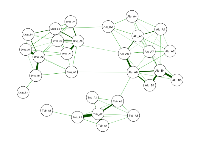
Note that although I kept using the term partial correlations, in the
Ising model, the exact meaning of the edge weights are log odds (as in
logistic regression). However, let’s think of it as a type of partial
relationship that is not bonded between -1 and 1.
#Take a look at edge weights
head(singSym$weiadj)
##           Alc_A1    Alc_A2    Alc_A3    Alc_A4    Alc_A5    Alc_A6    Alc_A7
## Alc_A1 0.0000000 0.4304911 1.2495301 0.6932798 0.1544171 0.0000000 0.3217432
## Alc_A2 0.4304911 0.0000000 0.8489614 0.1200658 0.5703120 0.8814447 0.6369553
## Alc_A3 1.2495301 0.8489614 0.0000000 0.4671812 1.3034016 0.0000000 0.8617096
## Alc_A4 0.6932798 0.1200658 0.4671812 0.0000000 0.0000000 0.0000000 0.6292706
## Alc_A5 0.1544171 0.5703120 1.3034016 0.0000000 0.0000000 1.6617679 1.1258700
## Alc_A6 0.0000000 0.8814447 0.0000000 0.0000000 1.6617679 0.0000000 0.4219963
##          Alc_B1    Alc_B2    Alc_B3    Alc_B4 Tob_A1 Tob_A2    Tob_A3 Tob_A4
## Alc_A1 0.000000 0.0000000 0.0000000 0.5669424      0      0 0.0000000      0
## Alc_A2 0.000000 0.0000000 0.0000000 0.0000000      0      0 0.0000000      0
## Alc_A3 0.000000 1.0989593 0.0000000 0.4509662      0      0 0.0000000      0
## Alc_A4 0.000000 0.9925397 0.0000000 0.2299741      0      0 0.0000000      0
## Alc_A5 0.629032 0.9733792 0.0000000 0.0000000      0      0 0.0000000      0
## Alc_A6 1.402567 0.0000000 0.4957041 1.3985314      0      0 0.7645253      0
##        Tob_A5 Tob_A6 Tob_A7 Drug_A1 Drug_A2  Drug_A3 Drug_A4 Drug_A5   Drug_A6
## Alc_A1      0      0      0       0       0 0.000000       0       0 0.0000000
## Alc_A2      0      0      0       0       0 0.000000       0       0 0.0000000
## Alc_A3      0      0      0       0       0 0.000000       0       0 0.0000000
## Alc_A4      0      0      0       0       0 0.000000       0       0 0.0000000
## Alc_A5      0      0      0       0       0 0.464126       0       0 0.0000000
## Alc_A6      0      0      0       0       0 0.000000       0       0 0.6730477
##        Drug_A7 Drug_B1 Drug_B2 Drug_B3 Drug_B4
## Alc_A1       0       0       0       0       0
## Alc_A2       0       0       0       0       0
## Alc_A3       0       0       0       0       0
## Alc_A4       0       0       0       0       0
## Alc_A5       0       0       0       0       0
## Alc_A6       0       0       0       0       0
The last demonstration paves the way for our next topic–mediating and moderating effect in network analysis. I will also explain why I choose R over Python for network analysis in the next article. See you next time. Have fun with your data. 🐱💻
Sin-Ying Lin
07/10/2021
Data can be retrieved from my github:
https://github.com/sin-ying-lin/blog_materials.git